Researchers have struggled for years to understand the conditions under which cooperation can emerge. The applications of such research can be found in industry, in society and in nature. As an applied mathematician the tool used in my research is a game called the prisoner’s dilemma . It’s origins go back to the 1950’s and it has been an ongoing research topic until today.
The prisoner’s dilemma is a two player game where the players can choose between two strategies, cooperation and defection. Since the 1980’s breakthrough, many are in search of the dominant strategy of the iterated version of the game; the iterated prisoner’s dilemma. Many explore not only the strategies themselves but also what makes them dominant and robust.
Since 2016 as part of my PhD, I was given the chance to work with a team of talented people on training a set of complex strategies and assessing their dominance and robustness. Some of the first outputs from this collaboration include:
- Evolution Reinforces Cooperation with the Emergence of Self-Recognition Mechanisms: an empirical study of the Moran process for the iterated Prisoner’s dilemma,
- Reinforcement Learning Produces Dominant Strategies for the Iterated Prisoner’s Dilemma.
The first paper, describes how several optimisation methods, such as genetic and particle swarm algorithms can be used to train dominant strategies of the iterated prisoner’s dilemma. The performance of the trained strategies were verified through tournament simulations. Most of the opponent strategies are from the literature. The second paper follows a similar approach but this time the robustness of the trained strategies is explored through an evolutionary process, called a Moran process.
In the first paper, it can be seen that iterated prisoner’s dilemma strategies can be represented with several different methods. Lookup tables, finite state machines and neural networks are all valid presentations of the strategies. One of the most beneficial ways is using finite state machines. A finite state machine, allows you to determine a player's next move by following a map of actions.
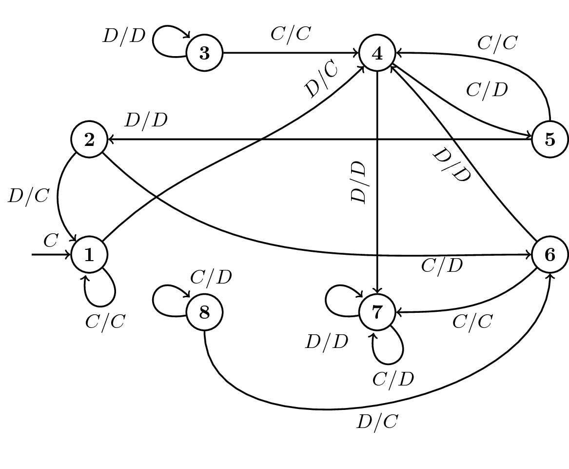
The image above is one of the trained strategies, an 8-state strategy, described in the second paper, represented using a finite state machine. Transition arrows are labelled O/P where O is the opponent’s last action and P is the player’s response. Note that the strategy’s first move, enters state 1, is always cooperation.
Drawing the finite state representation of the trained strategies found in both articles has been one my contributions to these papers. The strategies were given to my in python code with the following format:
fsm_transition =  [(0, C, 0, C), (0, D, 3, C),
                   (1, C, 5, D), (1, D, 0, C),
                   (2, C, 3, C), (2, D, 2, D),
                   (3, C, 4, D), (3, D, 6, D),
                   (4, C, 3, C), (4, D, 1, D),
                   (5, C, 6, C), (5, D, 3, D),
                   (6, C, 6, D), (6, D, 6, D),
                   (7, C, 7, D), (7, D, 5, C)]]
Note that writing the strategies this way is in line with how finite state machines strategies are encoded in the Python package Axelrod used in this work, see documentation.
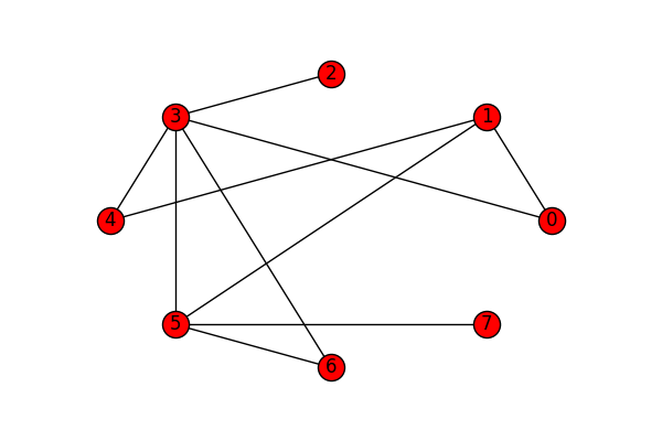
As a software developer I am very comfortable with the programming language Python. So on my first attempt to draw these strategies I used a Python tool called networkx. Networkx, allows me to generate a simple graph to find the best layout, using the library's already defined layouts.
>>> import networkx as nx
>>> G = nx.Graph()
>>> G.add_nodes_from(range(8))
>>> edges = [[0,  0], [0,3,],
             [1,  5], [1, 0,],
             [2,  3], [2, 2,],
             [3,  4], [3, 6,],
             [4,  3], [4, 1,],
             [5,  6], [5, 3,],
             [6,  6], [6, 6,],
             [7, 7],  [7, 5]]
>>> G.add_edges_from(edges)
>>> pos = nx.shell_layout(G)
>>> nx.draw(G, pos=pos, with_labels = True)
All of this leads to the Tikz code below:
\documentclass{standalone}

\usepackage{tikz}
\usepackage{standalone}
\usetikzlibrary{calc}

\begin{document}
    \begin{tikzpicture}
    \tikzstyle{state}=[minimum width=0.5cm, font=\boldmath];

    \node[circle, draw=black, thick]  (0) at (0,0) [state] {$1$};
    \node[circle, draw=black, thick]  (1) at ($(0)+(0,2)$) [state] {$2$};
    \node[circle, draw=black, thick]  (2) at ($(1)+(2,1.5)$) [state] {$3$};
    \node[circle, draw=black, thick]  (3) at ($(2)+(3,0)$) [state] {$4$};
    \node[circle, draw=black, thick]  (4) at ($(1)+(8,0)$) [state] {$5$};
    \node[circle, draw=black, thick]  (5) at ($(0)+(8,0)$) [state] {$6$};
    \node[circle, draw=black, thick]  (6) at ($(3)+(0,-4.5)$) [state] {$7$};
    \node[circle, draw=black, thick]  (7) at ($(2)+(0,-4.5)$) [state] {$8$};

    \coordinate[left of=0] (s);
    \draw (s) edge[out=0, in=180, ->, thick] node [above] {$C$} (0);

    \draw (0) edge[out=-45, in=-100, loop, thick] node [below] {$C/C$} (0);
    \draw (6) edge[out=-45, in=-100, loop, thick] node [below] {$C/D$} (6);
    \draw (6) edge[out=190, in=135, loop, thick] node [below, yshift=-0.5cm] {$D/D$} (6);
    \draw (7) edge[out=190, in=135, loop, thick] node [above, xshift=1cm] {$C/D$} (7);
    \draw (2) edge[out=190, in=135, loop, thick] node [left] {$D/D$} (2);

    \draw (2) edge[out=0,in=180,->,thick] node [above] {$C/C$} (3);
    \draw (3) edge[out=-35,in=170,->,thick] node [above right] {$C/D$} (4);
    \draw (5) edge[out=-135,in=0,->,thick] node [below] {$C/C$} (6);
    \draw (0) edge[out=45,in=-135,->,thick] node [above, rotate=45, xshift=2cm,
                                                  yshift=-0.5cm] {$D/C$} (3);

    \draw (1) edge[out=-45,in=180,->,thick] node [below right, xshift=2cm] {$C/D$} (5);
    \draw (1) edge[out=-135,in=135,->,thick] node [left] {$D/C$} (0);
    \draw (3) edge[out=-90,in=90,->,thick] node [above, rotate=90] {$D/D$} (6);
    \draw (4) edge[out=90,in=0,->,thick] node [above] {$C/C$} (3);
    \draw (4) edge[out=180,in=0,->,thick] node [above left, xshift=-2.5cm] {$D/D$} (1);
    \draw (5) edge[out=135,in=-45,->,thick] node [below, rotate=-45] {$D/D$} (3);
    \draw (7) edge[out=-90,in=-90,->,thick] node [below] {$D/C$} (5);
    \end{tikzpicture}
\end{document}
Note that the labels for the states of the finite state machine begin from 1 and not zero.
Furthermore, a small test was written to ensure that the transitions and actions of the strategies source code corresponded with the Tikz code.
>>> import collections
>>> import imp
>>> fsm_players =  imp.load_source('players', 'players.py')

>>> def tikz_line_to_transition(line):
...     """Parse a tikz line corresponding to an edge"""
...     current_state = int(line[line.index("(") + 1: line.index(")")])
...     next_state = int(line[line.index("(", line.index("(") +1) + 1: line.index(")", line.index(")") +1)])
...     input_action, output_action = line[line.index("{$") + 2: line.index("$}")].split("/")

...     return (current_state, input_action, next_state, output_action)

>>> def convert_tex_fsm(fsm_file):
...     fsm = []
...     with open(fsm_file, "r") as f:
...         for line in f:
...             if "\\draw" in line and not "(s)" in line:  # Pick out lines corresponding to an edge
...                 fsm.append(tikz_line_to_transition(line))
...     return fsm

>>> for i, tex_file in enumerate(["../tex/fsm_three.tex", "../tex/fsm_two.tex", "../tex/fsm_three.tex"]):
...     assert fsm_players[i].fsm.state_transitions == {transition[:2]:transition[2:] for  transition in
...     convert_tex_fsm(tex_file)}
All the work described in this blog was made possible due to an open source library called the Axelrod Python Library, http://axelrod.readthedocs.io/. I would like to thank the co authors of the papers mentioned in this blogs for making me part of this research,
Bonus: See Vince Knight’s blog post and Marc Harper’s blog post.