In game theory the game the prisoner’s dilemma has been used since the 1950’s to study interactions. Such as biological and social interactions. The prisoner’s dilemma is a two player non cooperative game where:
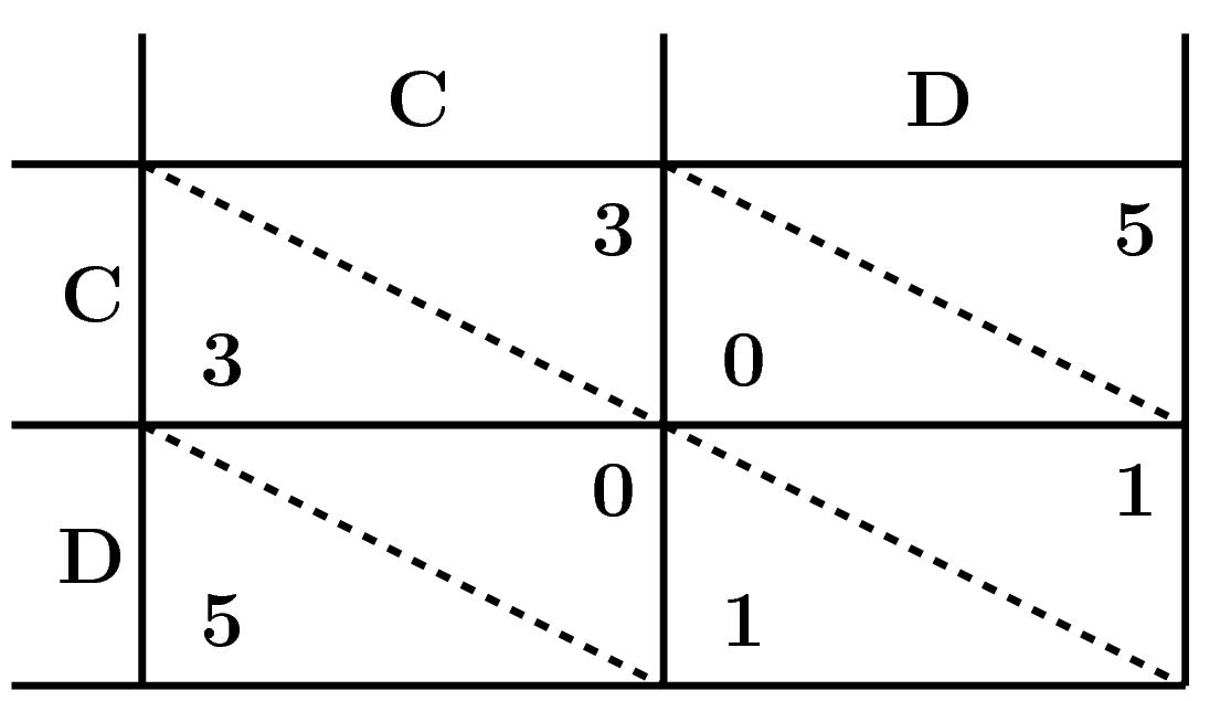
- Both players can choose to either Cooperate or Defect with each other.
- Both players are better of choosing Cooperation and receive a payoff of \(3\).
- Even so there is always a temptation for a player to Defect and gain a payoff of \(5\).
This can be described by the game matrix:
In the 1980’s, a political scientist called Robert Axelrod carried out a computer tournament of the iterated prisoner’s dilemma. In the iterated version of the game the players interact for a finite number of times and they are allowed access to the full history of the matches. Players can choose the size of history which they are going to use in deciding their next move.
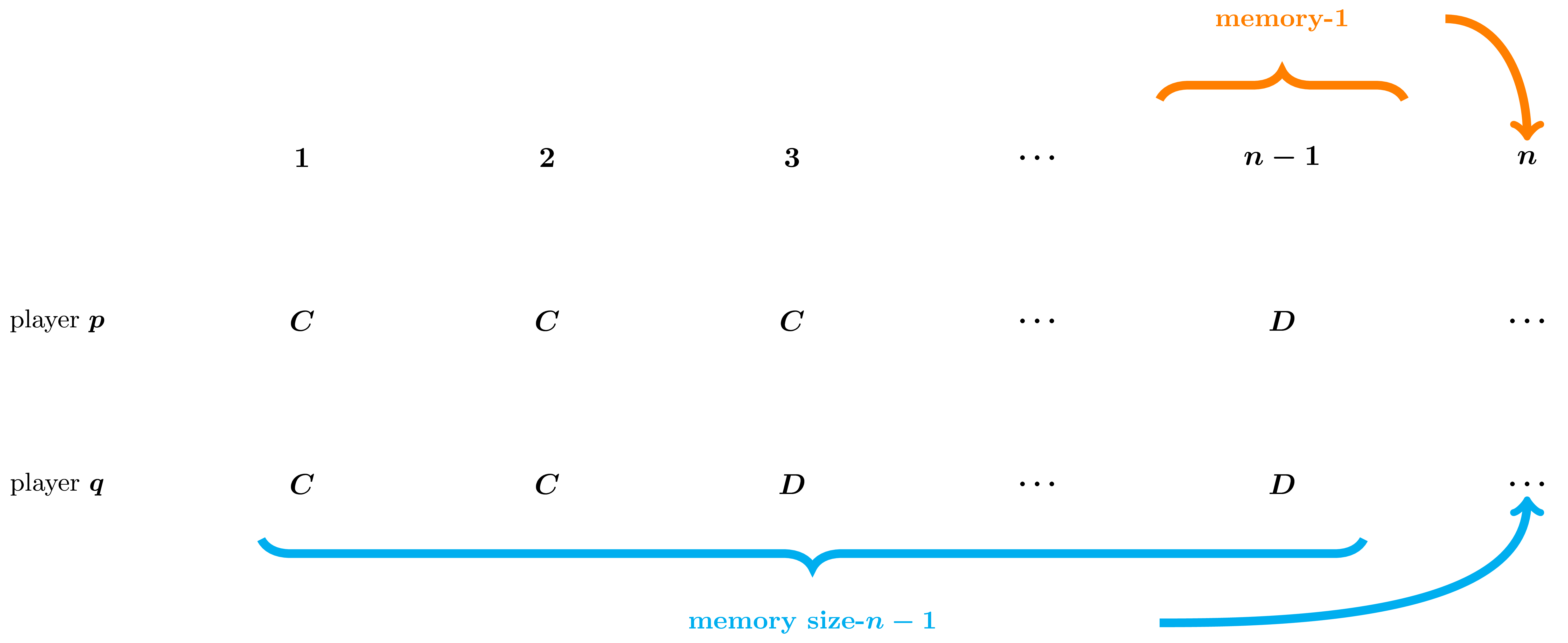
In 2012 Press and Dyson studied the iterated prisoner’s dilemma and focused on strategies that made use of the history of the previous round only. This set of strategies are called memory one strategies. When we only take into account a single turn of the game there are only four possible states that our player could possibly be in. These are \(CC, CD, DC\) and \(DD\).
A memory one strategy is denoted by the probabilities of cooperating after each of these states, \(p = (p_1, p_2, p_3, p_4) \in R_{[0,1]} ^ 4\).
Press and Dyson found a way for a memory one opponent \(p\) to manipulate an opponent \(q\) and they called these “manipulative” strategies, zero determinant strategies. Moreover, Press and Dyson stated that in a two player interaction, a player playing a zero determinant strategy can outdo any longer memory strategy. Concluding that in the iterated prisoner’s dilemma a longer memory size than 1 is not advantageous.
The purpose of my project is to show that memory one strategies have limitations. In order to achieve that I want to initially identify the best response \(p^*=(p_1, p_2, p_3, p_4)\) to a strategy \(q\). In essence answering the question:
What is the best memory one strategy against a given other memory one strategy?
A match between two memory one players \(p\) and \(q\) can be modelled as a stochastic process, where the players move from state to state. More specifically, it can be modelled by the use of a Markov chain, which is described by a matrix \(M\).
\[M = \begin{bmatrix} p_{1} q_{1} & p_{1} (- q_{1} + 1) & q_{1} (- p_{1} + 1) & (- p_{1} + 1) (- q_{1} + 1) \\\ p_{2} q_{3} & p_{2} (- q_{3} + 1) & q_{3} (- p_{2} + 1) & (- p_{2} + 1) (- q_{3} + 1) \\\ p_{3} q_{2} & p_{3} (- q_{2} + 1) & q_{2} (- p_{3} + 1) & (- p_{3} + 1) (- q_{2} + 1) \\\ p_{4} q_{4} & p_{4} (- q_{4} + 1) & q_{4} (- p_{4} + 1) & (- p_{4} + 1) (- q_{4} + 1) \end{bmatrix}\]Our players are assumed to move from each state until the system reaches a state steady. Thus in order to calculate the utility of our players we multiply the steady states of \(M\) with the payoffs of the game matrix.
More specifically, the first result discussed here is that the utility of player \(p\) against an opponent \(q\), denoted as \(u_q(p)\), can be written in a compact way:
\[u_q(p) = \frac{\frac{1}{2}p^TQ + c^Tp + a} {\frac{1}{2}p^T\bar{Q} + \bar{c}^Tp + \bar{a}}\]
where \(Q, \bar{Q}\) are matrices of \(4 \times 4\), and \(c, \bar{c}\) are \(4 \times 1\) vectors defined with the transition probabilities of the opponent’s transition probabilities \(q_1, q_2, q_3, q_4\).
Thus in order to answer our question, what is the best memory one strategy against
a given other memory one strategy?, we need to consider the following optimization
problem:
\[ max_{q}: u_q(p) \] \[st: \ p \in\mathbb{R}_{[0,1]}^{4}\]
Obtaining an analytical solution to this problem is not immediate. Thus in this blog post and as a second part of my work I considered a constrained version of the above problem. This was mainly done to get a better understanding of how to tackle the bigger problem.
More specifically, the constrained problem explored here is that of a set of memory one strategies where the transition probabilities of each state are the same. These are called purely random strategies and can be denoted as \(p = (p, p, p, p)\). Now our optimisation problem can be re-written as:
\[ \max_p: u_q(p) = \frac{n_2p^2 + n_1p +n_0 } {d_1p + d_0}\] \[ p_1 = p_2 = p_3 = p_4 = p \] \[ \ 0 \leq p \leq 1 \]
where \(n_2, n_1, n_0, d_1, d_0\) are constants defined with the transition probabilities of the opponent’s transition probabilities \(q_1, q_2, q_3, q_4\).
Determining \(p^*\) for a given \(q\) becomes simpler. It can be proven that obtaining the optimal random behaviour \(p ^ *\) reduces to a search over a small finite set. This is described by the following theorem:
Theorem 1. Optimisation of purely random player in a match
The optimal behaviour of a purely random player \((p, p, p, p)\) against a memory one opponent \(q\) is given by:
\[p^* = \text{argmax}(u_q(p)), \ p \in S_q,\]
where:
\[S_q = \{0, p_{\pm}, 1 | \begin{array}{l} 0 < p_{\pm} < 1, \
p_{\pm} \neq \frac{-d_0}{d_1} \end{array} \} \]
and \(p_{\pm}\) are the roots of \(\frac{du}{dt}\).
Computer trials have been performed to test the above theorem. The results are shown in the figure below,

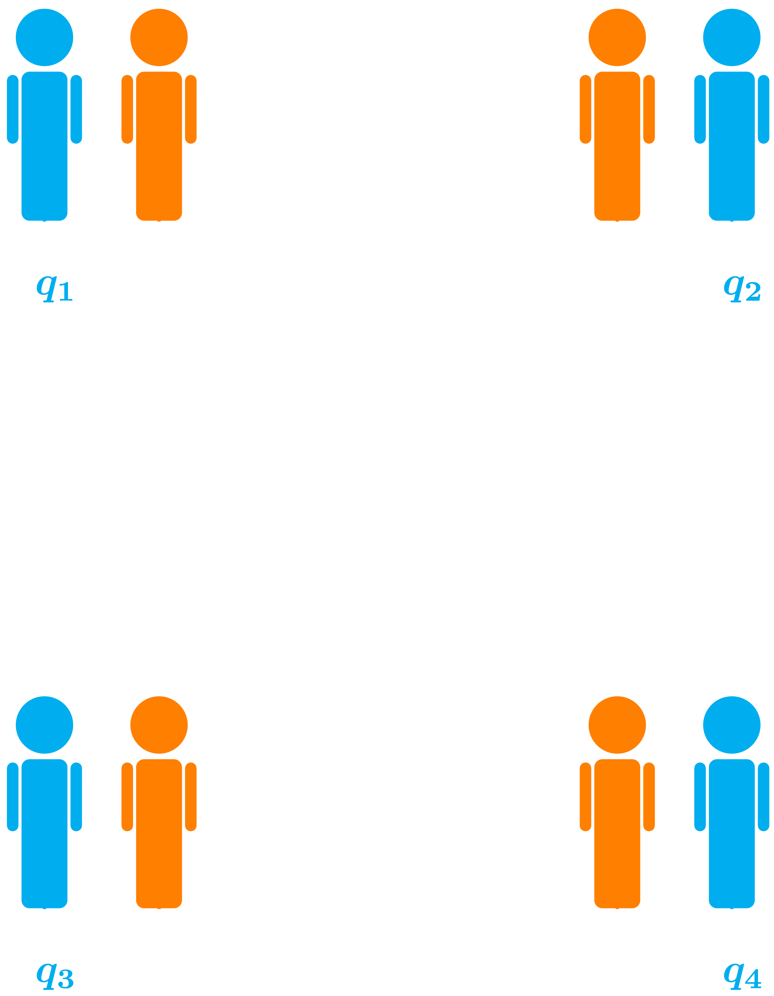
This approach can also be expanded on to consider multiple players \(q^{(1)}, q^{(2)}, \dots ,q^{(N)} \) and obtaining the optimal random behaviour \(p ^ *\) over a small finite set. In particularly this result is obtained by:
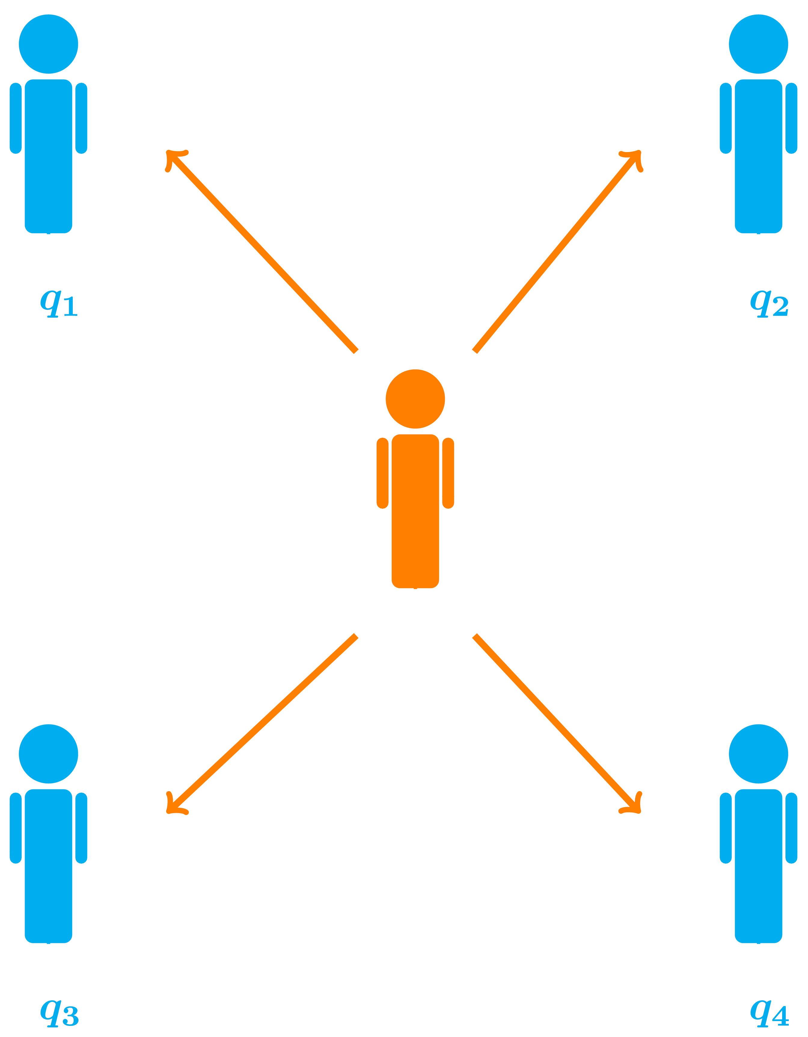
Theorem 2. Optimisation of purely random player in a tournament
The optimal behaviour of a purely random player \((p, p, p, p)\) in an \(N-\)memory one player tournament, \({q_{(1)}, q_{(2)} \dots,q_{(N)} }\) is given by:
\[p^* = \text{argmax}(\displaystyle \sum_{i=1} ^ {N} {u_q}^{(i)} (p)), \ p \in S_{q(i)},\]
where:
\[ S_{q(i)} = \overset{2N}{\underset{\lambda_i \neq \frac{do_i}{d1_i}}{\underset{i=1}{u}}} \lambda_i \cup {0, 1} \]
and
\(\lambda_i\) are the eigenvalues of the companion matrix of \(\frac{du_{q(i)}(p)}{dp}.\)
Note the size of candidate solutions is \( 1 \leq|S_{q(i)}| \leq 2N + 2\).
Computer trials have been also been run to test the above theorem. The results are given by,
Two things are captured by Theorem 2. Initially it can be seen that optimising against the mean utility can not be captured by optimising against the mean opponent. Secondly and more importantly it is shown that a strategy with memory greater than 1 (evolved) out performs the optimal purely random player.
This where the limitations of memory one lies. In interactions with multiple opponent it can shown that having a larger memory, essentially being a bit smarter, can be advantageous.
The next step of this work, which is currently in progress, is to generalized both theorems to memory one players! This will be done with the assistance of resultant theory, which will allow me to solve multivariate systems, but I will leave this for another blog post.
p.s. This blog post accompanies my poster The power of memory which was presented in the SIAM UKIE Annual Meeting 2018.